
Bonding or Antibonding?#
In this example we show how to differentiate between a bonding and antibonding MO for two chosen fragments. As a system we chose the homolytic bond-cleavage of the carbon-chloride bond in chloroethane calculated at the ZORA-OLYP/TZ2P level of theory.
In general, to know if an MO has bonding or antibonding character for two chosen fragments we calculate the bond order
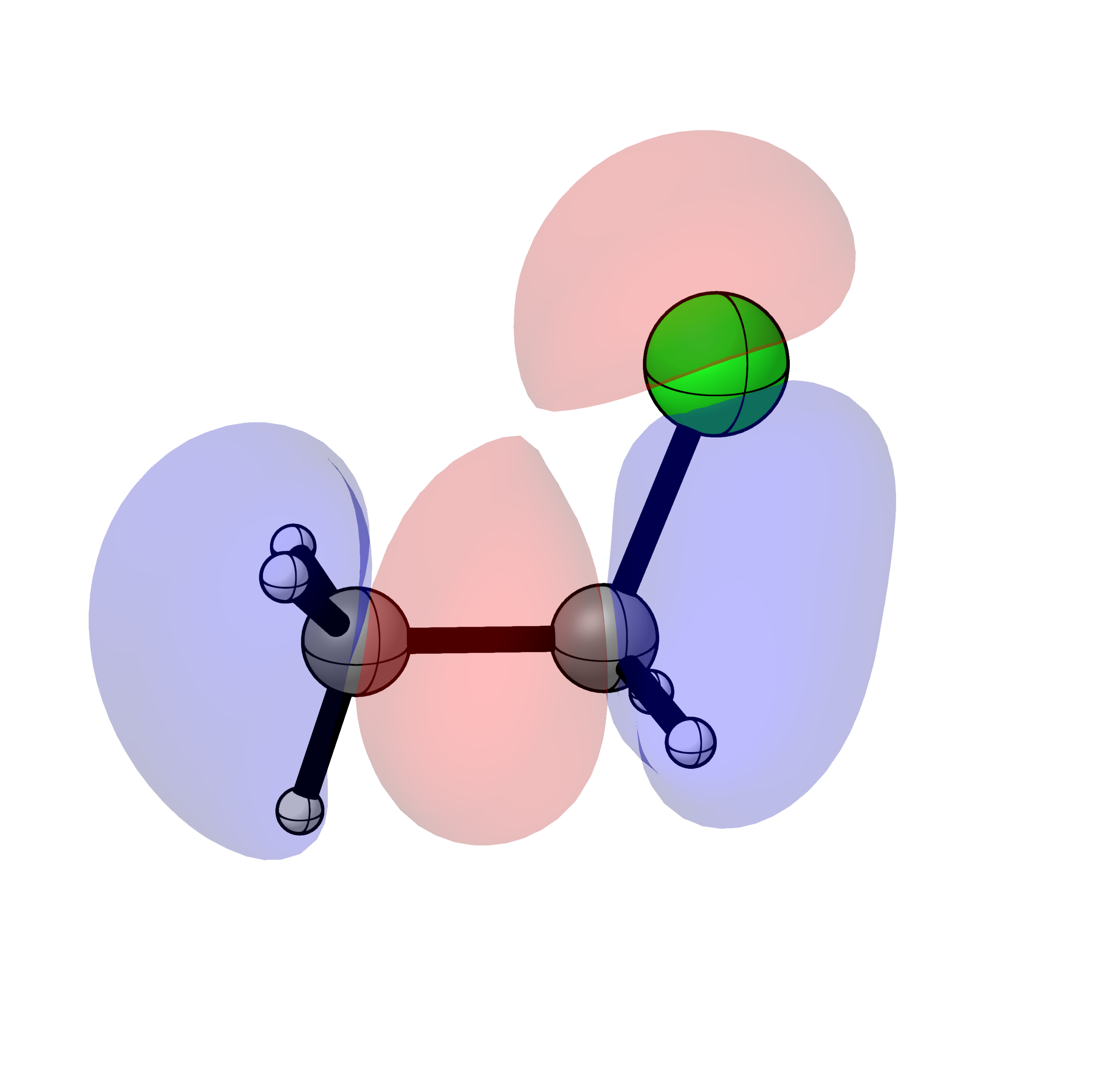
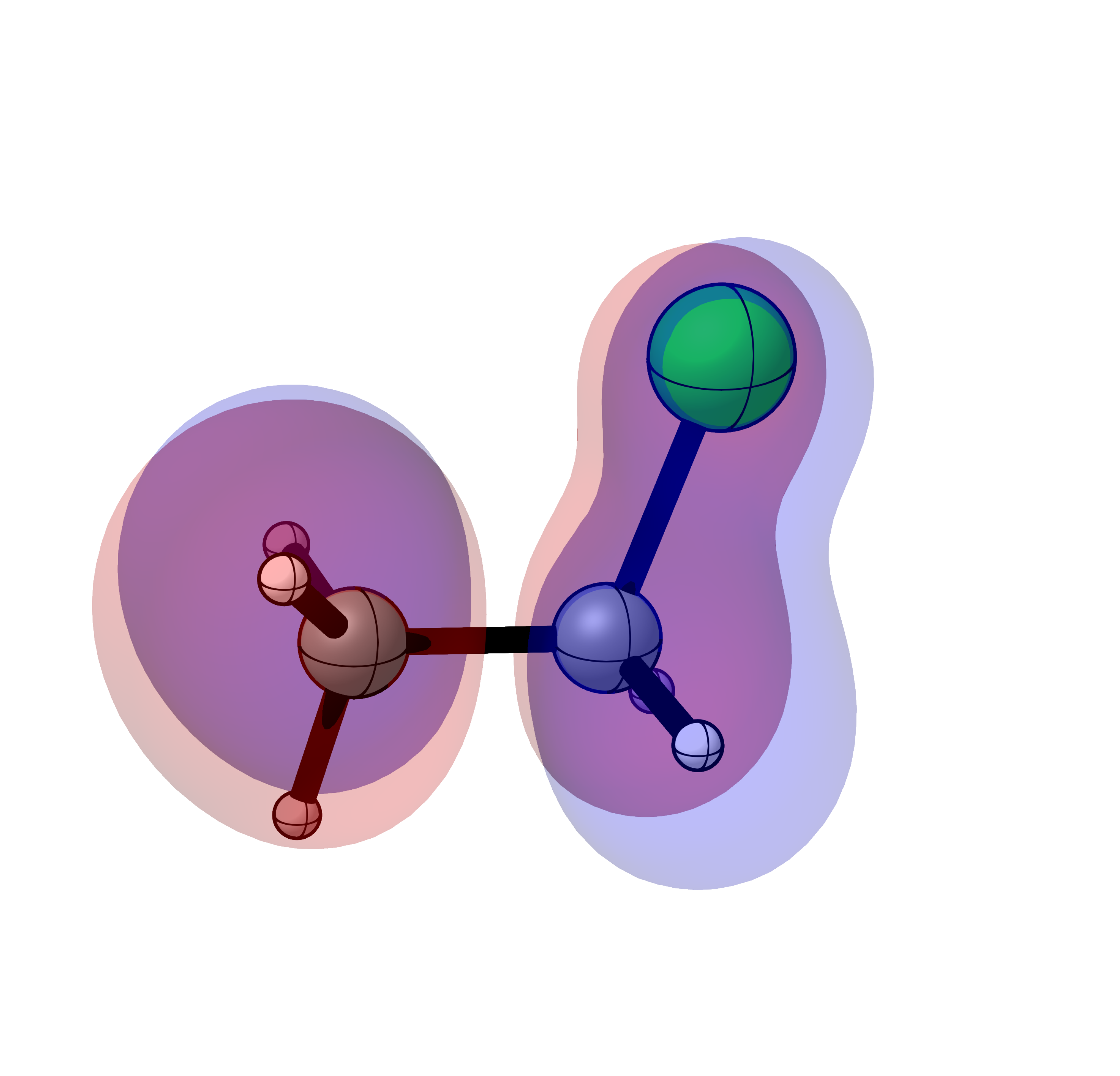
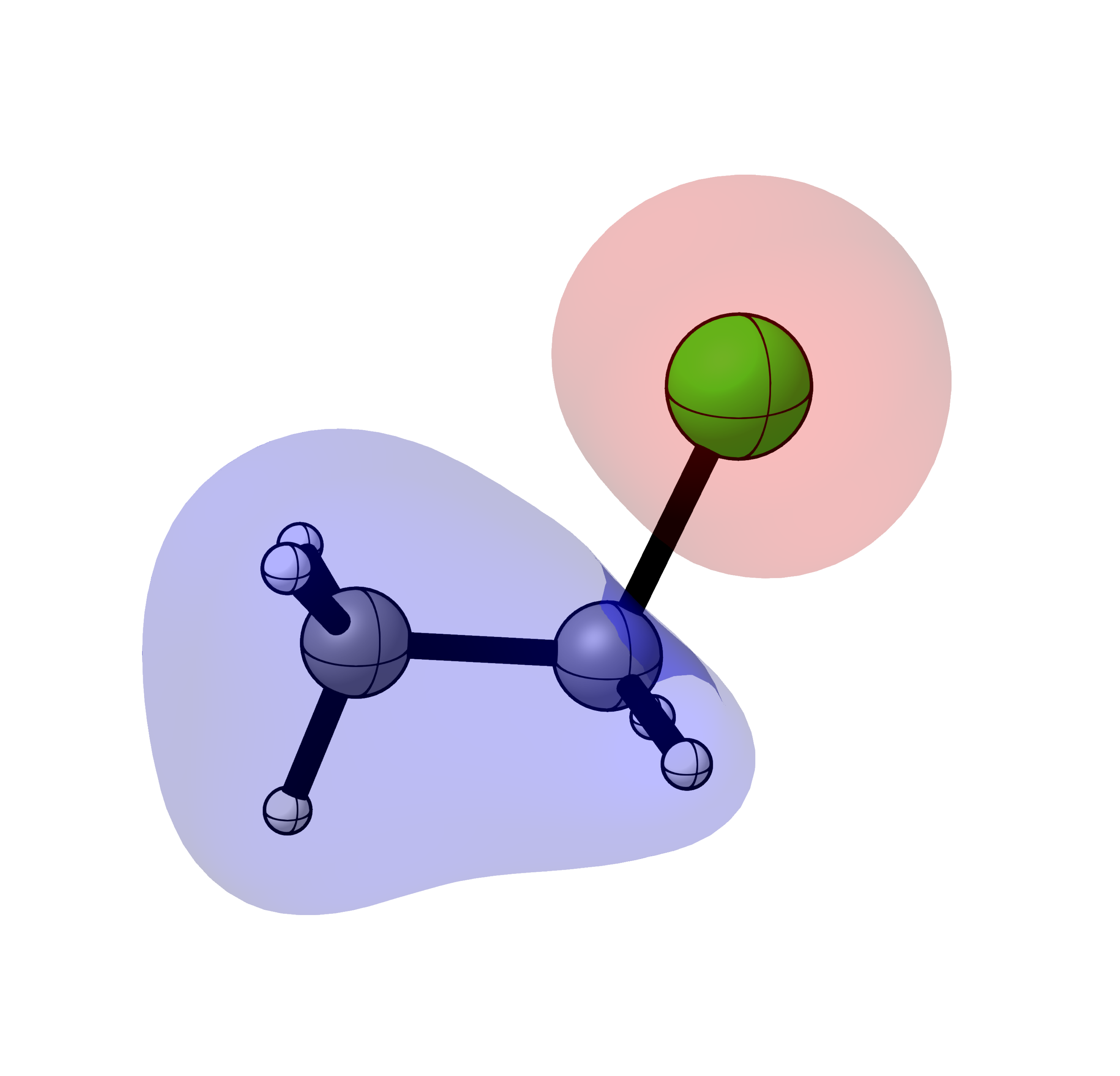
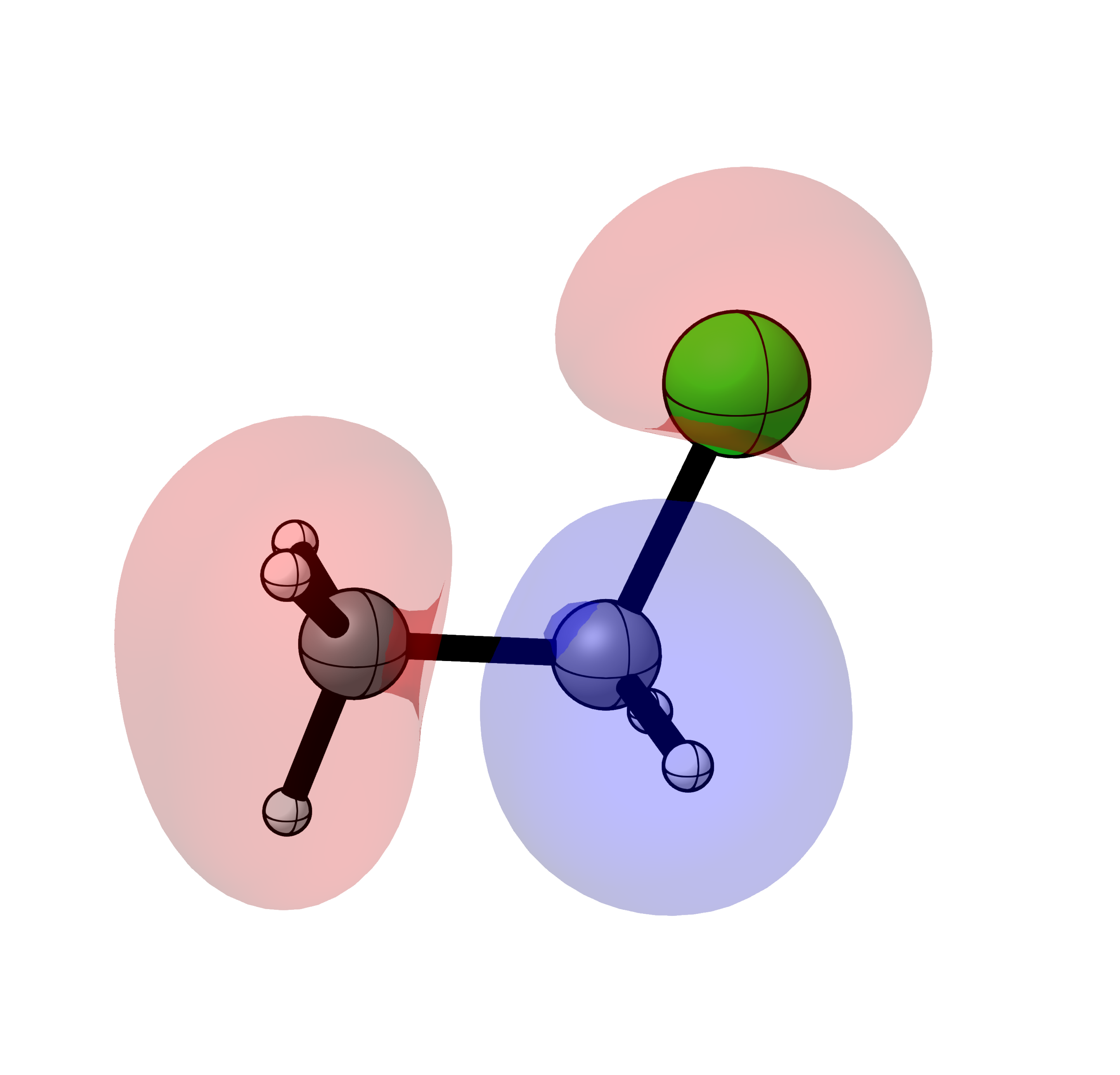
where \(\Psi_i\) is the MO of interest with occupation \(N_i\) and \(\{\psi^A\}\) and \(\{\psi^B\}\) are the sets of SFOs from fragment A and B respectively. \(\langle \psi_j^A | \Psi_i \rangle\) is the projection coefficient of \(\psi_j^A\) onto the MO and \(\langle \psi_j^A | \psi_k^B \rangle\) is the overlap between the SFOs. A negative value for \(\textrm{BO}(\Psi_i)\) is antibonding character and a positive value bonding character. The magnitude of \(\textrm{BO}(\Psi_i)\) indicates how strong the bond or antibond is. If the value is close to zero we are likely dealing with a non-bonding combination.
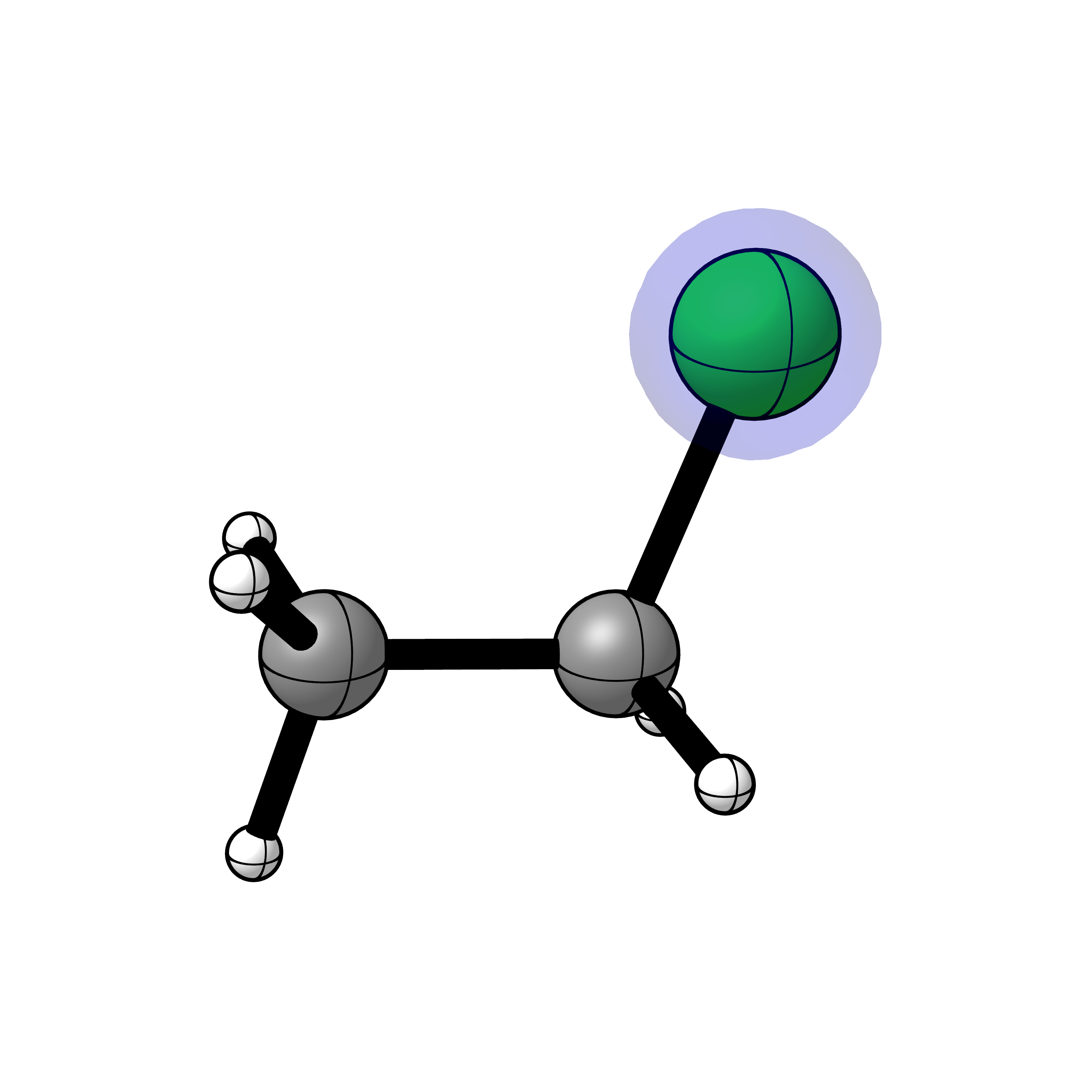
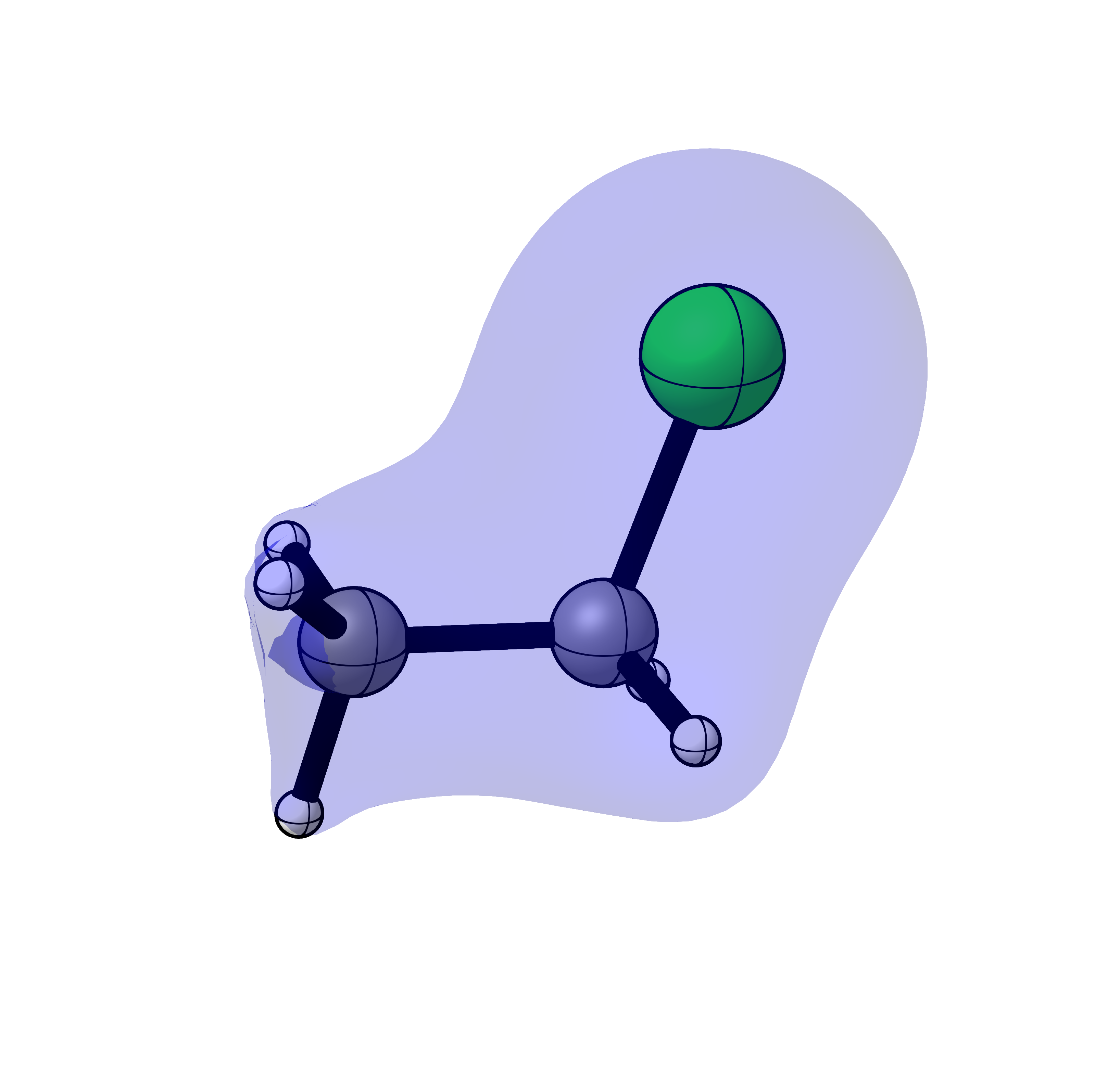
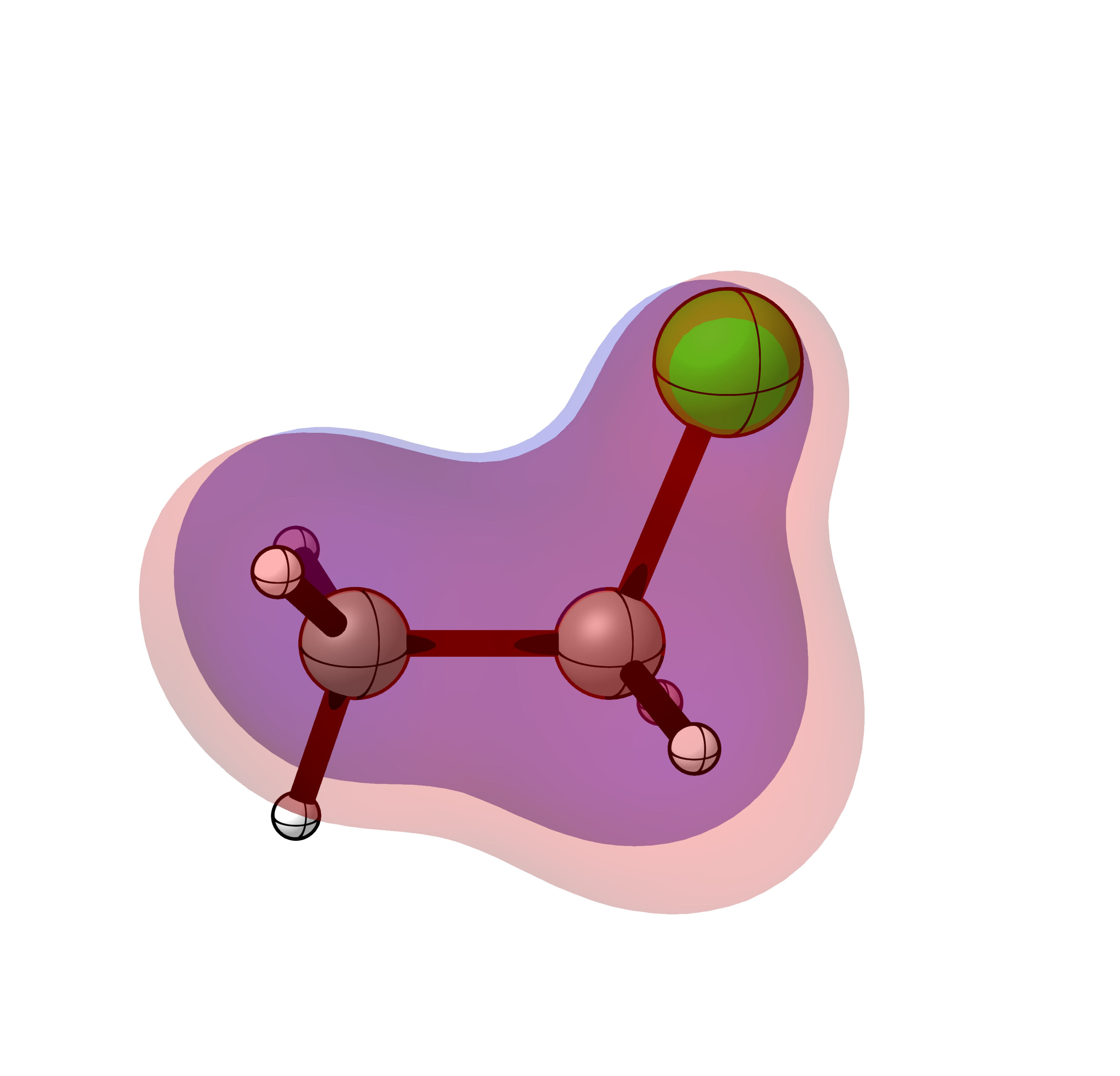
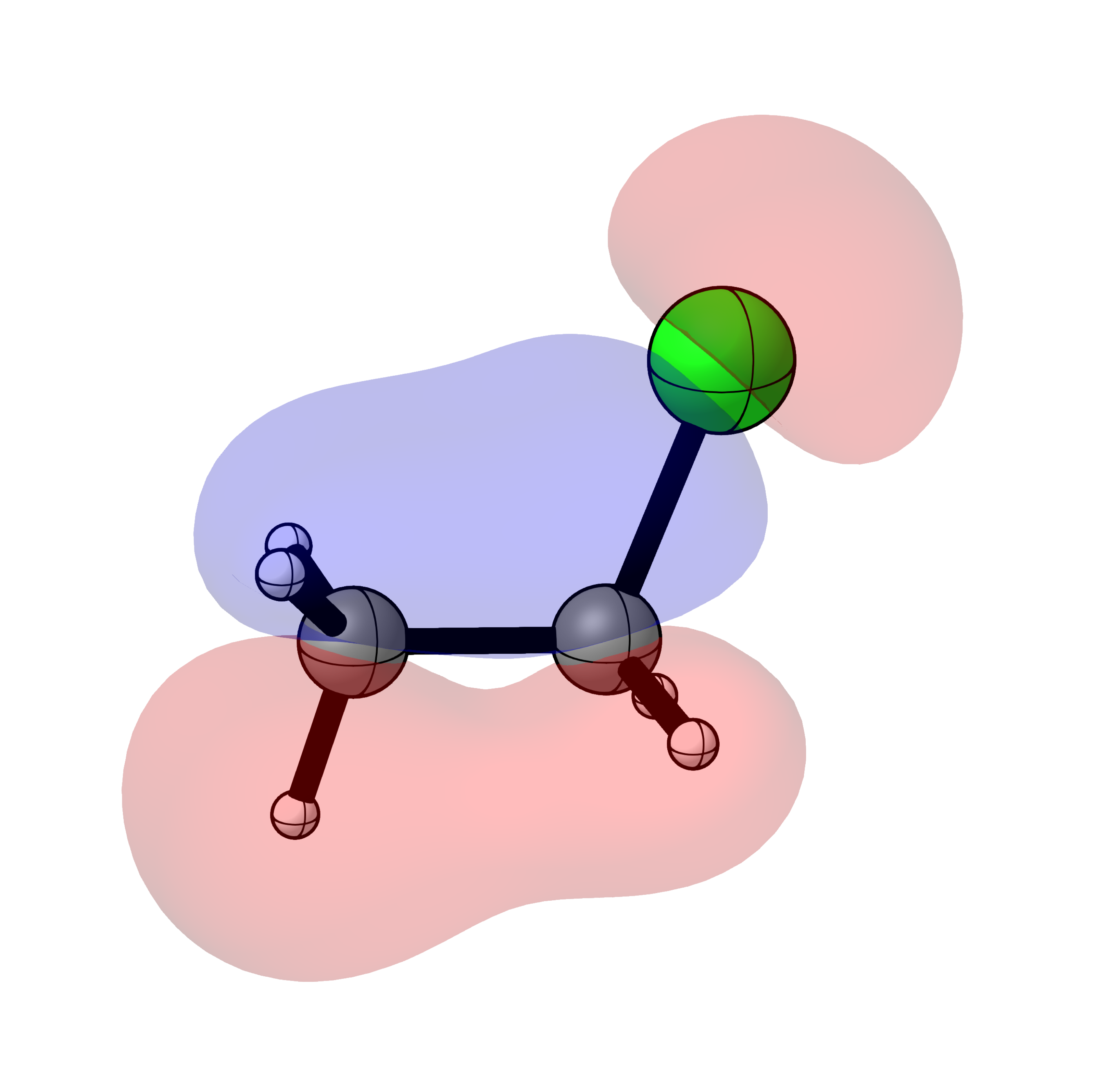
Calculating the bond order for the MOs of chloroethane yields the following bonding and antibonding MOs that have a bond order strength of 0.001 or greater:
|
|
|
MO 4A |
MO 8A |
MO 11A |
|
|
|
MO 12A |
MO 13A |
MO 14A |
|
|
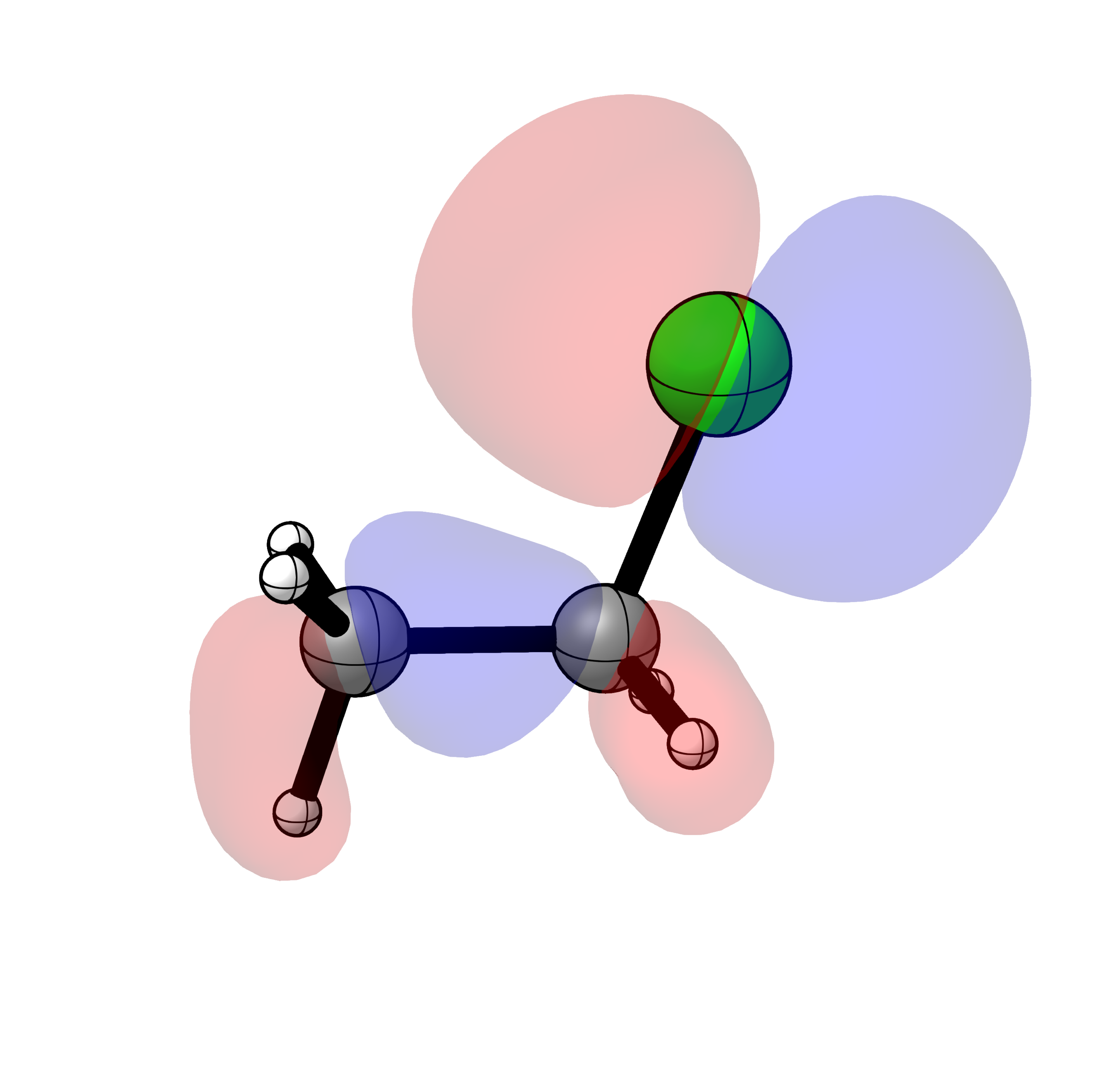
|
MO 9A |
MO 10A |
MO 16A |
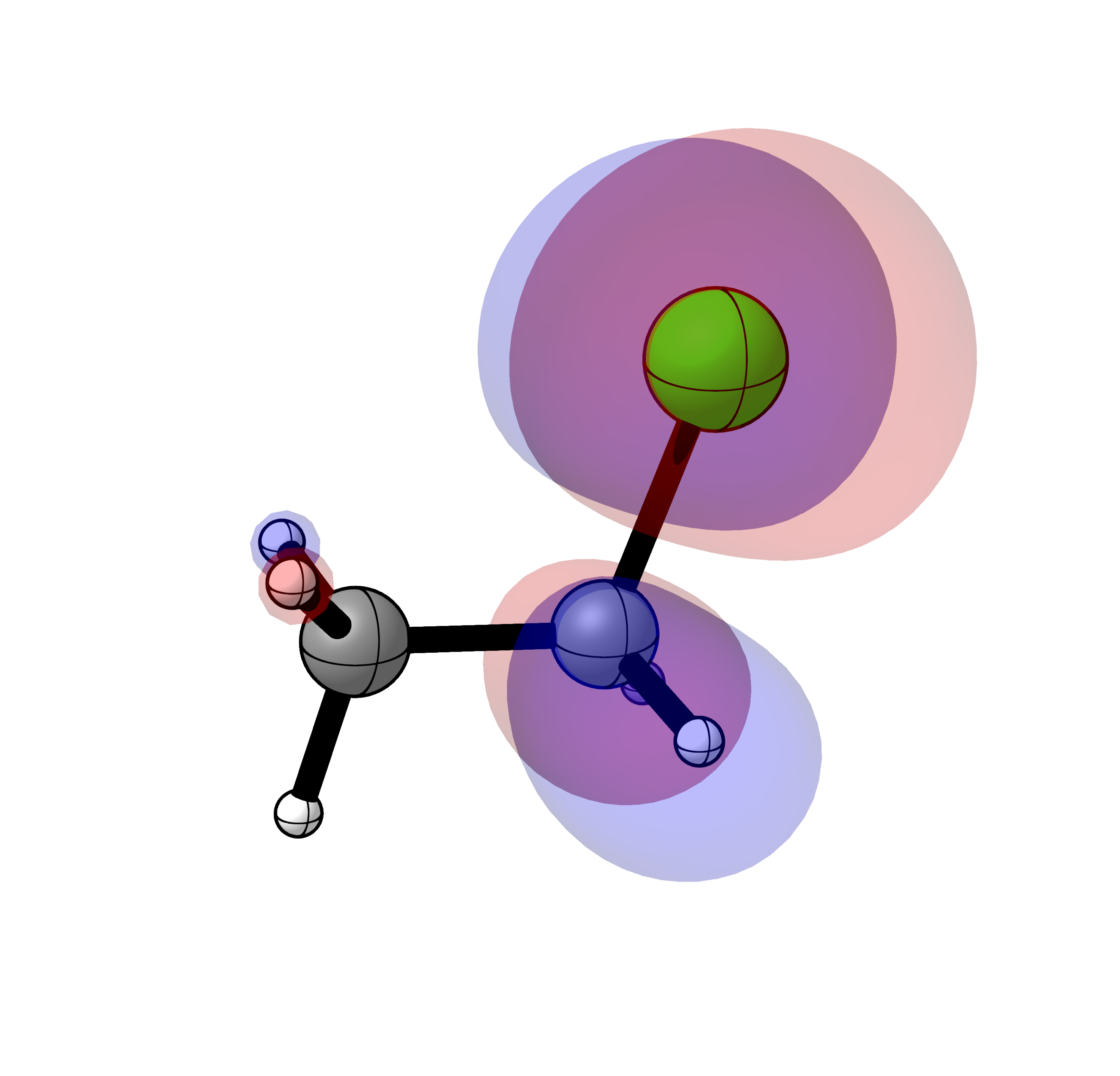
|
||
MO 17A |
Download bonding.adf.rkf
Download bonding.py
'''
This example shows how to find bonding and anti-bonding orbitals.

This example uses an ADF calculation on chloroethane
calculated at the OLYP/TZ2P level of theory.
The C-Cl bond was homolytically cleaved.
'''

import pyorbb


def bond_order(mo, fmos1, fmos2):
	'''
	This function calculates the bond order for an MO between two sets of FMOS.
	The bonding order is the sum of all overlap populations between the two
	sets of FMOs.
	'''
	total = 0
	for fmo1 in fmos1:
		c1 = fmo1.coefficient(mo)
		for fmo2 in fmos2:
			c2 = fmo2.coefficient(mo)
			S = fmo1.overlap(fmo2)
			# this is the overlap population between fmo1 and fmo2
			total += 2 * mo.occupation * c1 * c2 * S

	return total

# load the orbital data
orbs = pyorbb.Orbitals('bonding.adf.rkf')

# split FMOS between the two fragments
fmos_fragment1 = orbs.fmos.filter(fragment='LeavingGroup')
fmos_fragment2 = orbs.fmos.filter(fragment='Substrate')

# to simplify we only consider one spin type for the MOs
mos = orbs.mos.filter(spin='A')

rows = []
total_bond_order = 0
# go through each MO and calculate the score
for mo in mos:
	score = bond_order(mo, fmos_fragment1, fmos_fragment2)
	total_bond_order += score

	# if the score is too low we don't show it
	if abs(score) < 1e-3:
		continue

	# if the score is high enough we write a new string to be printed later
	rows.append([mo, score > 0, score])

# add a total row
rows.append(['Total', total_bond_order > 0, total_bond_order])

# print the gathered data
print('   MO  Bonding?  Score')
print('──────────────────────')
for mo, bonding, score in rows[:-1]:
	print(f'{str(mo):>5}  {str(bonding):8} {score: .3f}')
print('──────────────────────')
print(f'{str(rows[-1][0]):>5}  {str(rows[-1][1]):8} {rows[-1][2]: .3f}')
The expected output is as follows
   MO  Bonding?  Score
──────────────────────
 4A_A  True      0.001
 8A_A  True      0.183
 9A_A  False    -0.067
10A_A  False    -0.009
11A_A  True      0.052
12A_A  True      0.072
13A_A  True      0.056
14A_A  True      0.027
16A_A  False    -0.073
17A_A  False    -0.088
──────────────────────
Total  True      0.154